
In this video and blog, we take a look at a conjugate heat transfer problem
with both convection and conduction using
SOLIDWORKS Flow Simulation.
Here are the steps used to set up the analysis.
Flow Simulation is a computational fluid dynamics (CFD) tool that operates
directly inside of SOLIDWORKS. You’ll need both
SOLIDWORKS and SOLIDWORKS Flow Simulation installed, with the Flow Simulation add-in
enabled, to follow along with this guide.
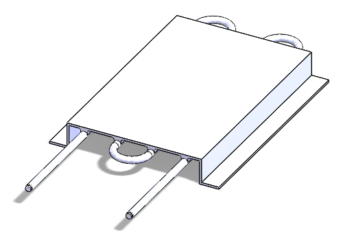
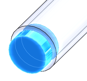
The first step is to get the geometry ready. For this cold plate, lids are
needed at both ends of the cooling tube. This allows the inside of the tube to
be defined as a separate internal fluid volume.
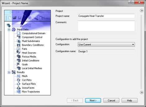
Next, I’ll create the Flow Simulation project using the Wizard. From the
Flow Simulation menu, I’ll select Project, Wizard. I’ll name the
project “Conjugate Heat Transfer” and choose to use the current configuration.
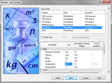
I’ll set my unit system as SI (m-kg-s) and change the unit for
temperature to °C.
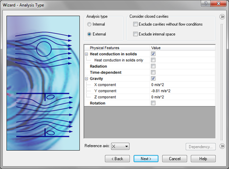
The analysis type is External because we want to consider the air
surrounding the model. I’ll turn on Heat conduction in solids and
Gravity, and confirm that Y component -9.81 m/s^2 is the correct
direction and value for this analysis.
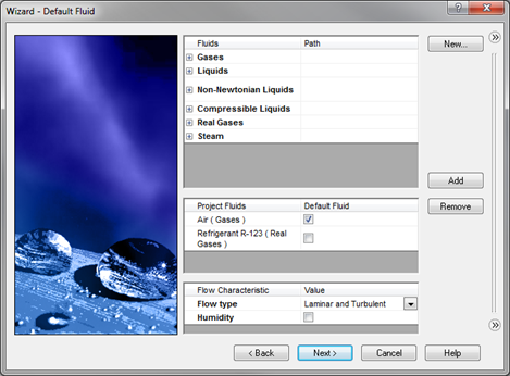
Air (Gases) and Refrigerant R-123 (Real Gases) are pre-defined
and can be added as the project fluids. I’ll make sure that the checkboxes are
set so that Air (Gases) is the Default Fluid.
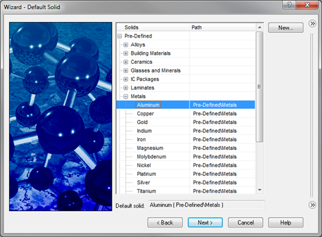
Aluminum is pre-defined under Metals and can be set as the
default solid.
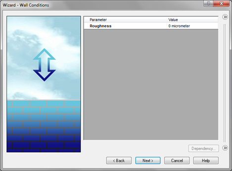
I can accept the default value of 0 micrometer for Roughness and
assume smooth walls.
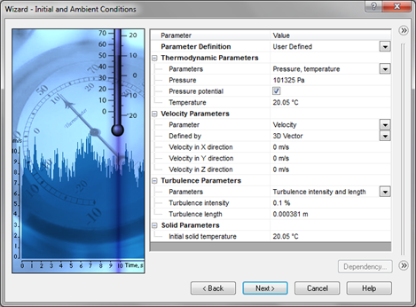
And I’ll accept the default values for the initial conditions.
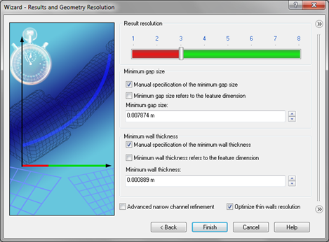
I’ll keep the Result resolution relatively low to start with and set it
to 3, and I’ll enter 0.007874 m for the
Minimum gap size and 0.000889 m for the
Minimum wall thickness, which correspond to the inner diameter and
thickness of the tube. I’ll click Finish and work my way down the Flow
Simulation analysis tree.
The automatically generated computational domain is bit larger than I need so
I’ll right-click Computational Domain, select Edit Definition,
and enter the following values.

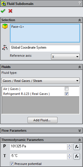
A fluid subdomain needs to be defined to set the fluid inside the tube as the
refrigerant. I’ll right-click Fluid Subdomains and select
Insert Fluid Subdomain. I’ll select an internal face of the tube, set
the checkbox next to Refrigerant R-123 (Real Gases), and enter
101325 Pa and -5 °C for the Thermodynamic Parameters.
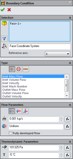
Next up are the boundary conditions. I’ll right-click
Boundary Conditions and select Insert Boundary Condition. I’ll
select the inner face of the inlet lid and define an
Inlet Mass Flow with the parameters shown below.
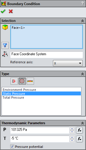
And I’ll insert another boundary condition on the inner face of the outlet lid
and define a Static Pressure as shown below.
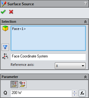
A surface source can be used to generate heat at the top of the plate. From
the Flow Simulation menu, I’ll select Insert, Surface Source.
I’ll select the top surface of the plate and enter a
Heat Generation Rate of 200 W.
The last thing to do before running the project is to define the goals. I’ll
right-click Goals, select Insert Global Goals, and select the
Max checkboxes for the Temperature (Fluid) and
Temperature (Solid).
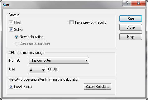
And that’s it. The project is ready to run. I’ll right-click the project name,
select Run, ensure that the checkbox for Solve is selected, and
click the Run button. This initial setup is a good start for this
problem, but it’s of course a great idea to refine the setup after running the
analysis and taking a look at the results.
Once the analysis is complete, there are many ways to investigate the results.
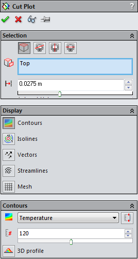
As an example, I’ll create a cut plot to view the temperature of the coolant
in the tube. I’ll right-click Cut Plots and select Insert. I’ll
set my plot halfway through the tube, 0.0275 m above the
Top Plane, and choose to show Temperature Contours.
The plot shows that the coolant rises from its initial temperature of -5 °C to
a maximum of about 80 °C by the end of the tube.
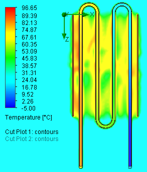
Better performance, especially at the left half of the cold plate, could
likely be achieved by reducing the temperature increase of the coolant, so
increasing the flow rate through the tube might be a good idea.
SOLIDWORKS Flow Simulation allows for changes to the design and analysis to be
cycled through at the same time and it shouldn’t be too long before an
improved cold plate is nailed down.
I hope you found this conjugate heat transfer example useful. If you have any
questions, please leave a comment and let us know.

Hello. I have to do a similar simulation, but with solar radiation. It’s a box of aluminium, with a glass on top. In the box there is only air! Do you know how I can do it? Thank you very much!
Hi, SW Expert !!!
I am a SolidWorks users in Korea.
According to your lesson and I study to solidworks flow simulation.
I want to insert, and the temperature (solid) does not find to goals from checkbox.
Tell us what to do. Note that I am using solidworks 2015.
Thanks for your good job.
from korea
Sorry for the very slow response. It appears our comment alert system hasn’t been working.
Antonio, you can definitely include solar radiation. In your analysis settings, simply enable the “Radiation” option and then enable the “Solar radiation” option. You can define solar radiation by your location on the earth and time, direction and intensity, or azimuth and altitude. Check out the Flow Simulation tutorials for more tips on setting up radiation.
Hyunjoo, if I understand your question correctly, you’re not seeing options for “Temperature (Solid)” when creating goals. Please ensure that you have enabled “Heat conduction in solids” in your analysis settings. The “Temperature (Solid)” options are only available when running a thermal study.
Hello,
I’m new in flow simulation. I’m trying to simulate an assembly with a duct and a heat sink. The heat sink is inserted in the duct by the part of the fins in order to capture the heat flow through the duct.
This is an internal analysis with default outer wall condition (heat transfer coefficient =7w/m2K).
The heat sink is aluminium and de duct Aisi 305.
When I simulate it, the temperature through de heat sink is uniform. It means, the internal temperature is 350°, the fins are at 230 approximately and the Base is 229. How can I fixed it?
Best regards
Andrés, this sounds a bit too detailed to handle through comments. If you’re a Hawk Ridge Systems customer, please give us a call at 877.266.4469 and we can help you out with your analysis. Otherwise, please get in touch with your local VAR.
Hi Mr Terence
I’m currently working on my Final Year Project (FYP) for my bachelor. Im facing one problem that particles in fluidized bed suppose have different temperature after being added heat and also contributed by collision of the particles. Somehow, my temperature of the particles remain same temperature. How can I solve this problem? Thank you in advance 🙂
Xiao Fen, you should be able to see a change in the temperature of your particles provided that they are a different temperature from the fluid when injected. The initial particle temperature can be defined either as an absolute value or relative to the temperature of the fluid. Also, make sure that you are looking at a plot of Particle Temperature when post-processing. Beyond these general tips, it’s hard to advise on your particular analysis without more details. If you’re a Hawk Ridge Systems customer, please give us a call at 877.266.4469 and we can help you out with your analysis. Otherwise, please get in touch with your local reseller.
Hey
My problem is a solar dish concentrate reflects radaiton of sun to coil with internal flow the temperature dose not raise and there is no radaiton
Hello Terence,
Thanks for the very elaborate way of setting up the problem and solving it. It is really helpful, specially for the first time users.
I would like to ask about a simple problem of heat transfer. We have a pipe which (around 80 mm long) and it is connected to another body at one end. at the other end we need to do welding. We would like to simulate this using solidworks and would like to see the temperature profile with time. This is needed to insure that due to welding, the other end of the pipe doesnt become too hot so that the components might fail.
Most important is to know the time in which the temperaure will become too high (say a value) that isnt acceptable.
any help is deeply appreciated.
Anurag, that sounds like a good application for some thermal analysis. It’s hard to advise on any specific setup details through blog comments through. If you’re interested in getting some more in-depth help, please give us a call and our analysis services team would be happy to discuss.
HELLO
Dear sir , i have some questions about flow simulation,i am using Solidworks 2020,and also i did a solver part.after that, i check out different plots.
my question is this after finish the solver window i can check different iteration,and also can you tell me after this all procedure i can see numaricle results and.
thanks for understanding.
Regards.
Azeem